Importing A Database Table Into Microsoft Excel.
The following instructions can be used to set up a Microsoft Excel spreadsheet to display information dynamically linked from a data table in the Acctivate database. The data can be refreshed to view real-time information from Acctivate.
- Create a new spreadsheet in Microsoft Excel
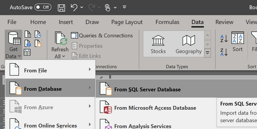
- Click the Data tab (at the top), then click Get Data and select From SQL Server
3. Connect to Database Server
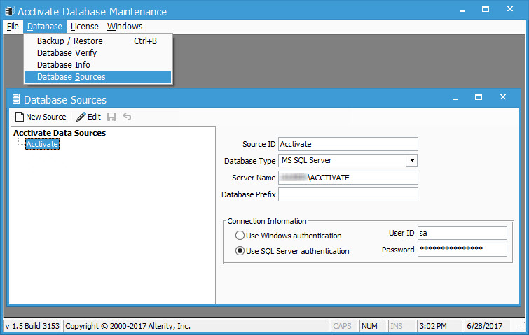
- Enter the Acctivate SQL Server name. You can find the SQL Server name by looking at “Database Sources” in the Acctivate Database Maintenance utility.
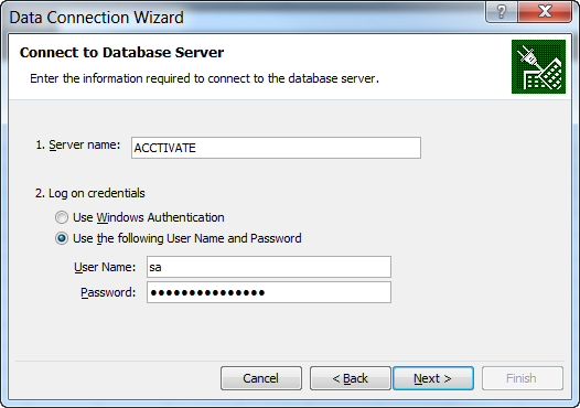
- Enter the SQL Server User ID and Password. The User ID is typically sa . You will need to obtain the password from the Acctivate Support Team if you don’t have the password for the sa account. Click Next to proceed.
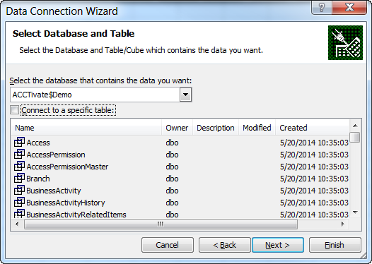
4. Select Database and Table
- Select the “ACCTivate$xxxxx” database (replacing xxxxx with your company). In this example, we’ll use the ACCTivate$Demo database.
- Un-check “Connect to a specific table” to include all tables, then click Next.
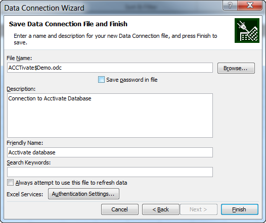
5. Save Data Connection File and Finish
- Type a brief Description, like “Connection to Acctivate database”, then click Finish.
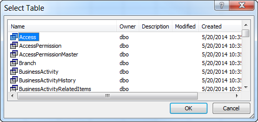
6. Select Table
- Select a Table or View to display on the worksheet. Please check out our list of data views that are available.We recommend that you use a database VIEW that does not begin with the “tb”prefix. The internal tables use the “tb” prefix and are subject to change.Using the database views will minimize the possibility of changes to the database that require an update to the spreadsheet.
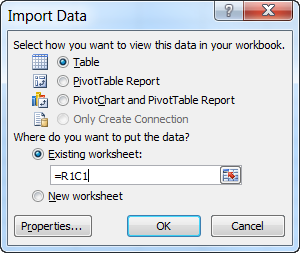
7. Import Data
- Typically, you will want to simply display the data into the Excel as a Table . However, advanced options, such as PivotTable Report are very powerful tools.
- Using the default “Existing worksheet” option will place the data into the worksheet, starting at the selected cell (typically $A$1)
- Click OK to load the table data
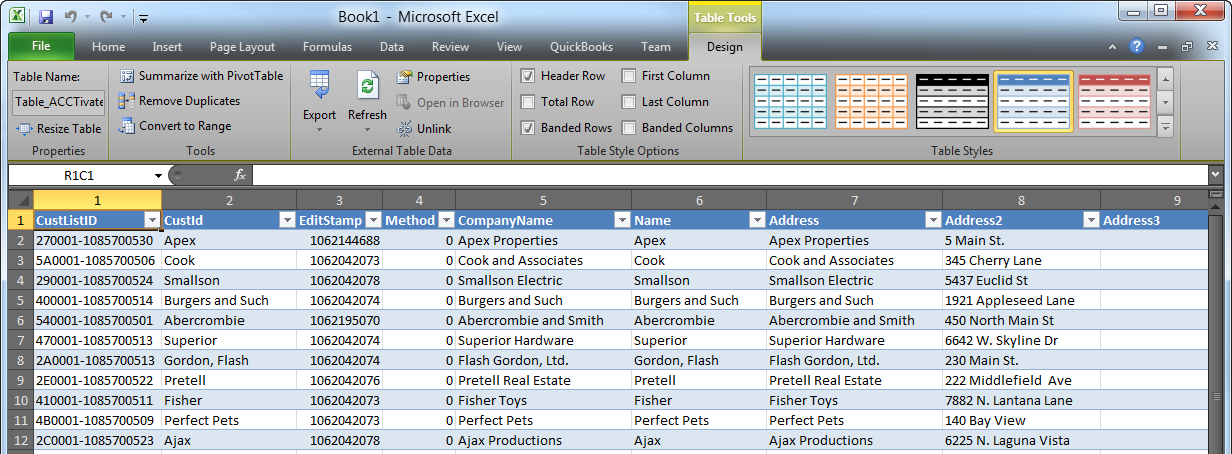
At this point, you should see a data grid in Excel containing information from the selected Acctivate data table.
