Stopping Excel from Changing Numbers to Dates or Scientific Notations.
We all know that Excel can be a powerful tool, however in an effort to anticipate the need of a user, Excel can also make it difficult to create spreadsheets for importing data into Acctivate QuickBooks Inventory Software. You may have entered a string of numbers in Excel only to find they were reformatted to a date or something else and no longer display what you intended. Importing or updating records in a database most often the data must match 'exactly'. Therefore when Excel changes the format of your import data your import will fail. This can be extremely frustrating but do not worry you have a few options to easily correct it.
The Apostrophe Method
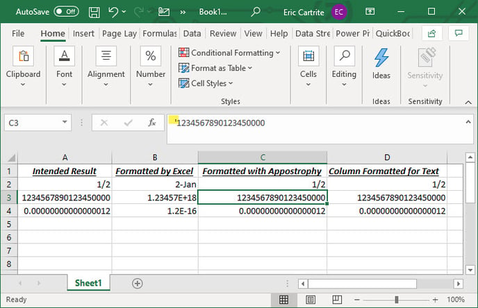
By placing an Apostrophe ( ' ) preceding the number, you will prevent Excel from reformatting the number and display the number exactly how you have it entered.
Example:
- Entering '1/2 into a cell it will prevent Excel from making your fraction a date.
This method means that even if someone were to change the cell formatting back to General and tries to edit a cell it will continue to look the same instead of being auto-formatted by Excel.
- Type an Apostrophe in the Cell
- Enter the number as you want it to display and press Enter
- Now the numbers should display and import correctly
- This will allow you use MATCH and VLOOKUP functions in Excel (Apostrophe will be ignored)

Format as Text Method
The second most common method to simply format the entire worksheet or a group of cells as Text before you enter your data. Formatting cells to display as text will make Excel display the data exactly as it has been entered. (Remember to format your cells Before you input your data)
- Select the entire sheet or a group of cells
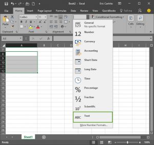
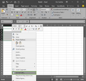
- Next you can either 'Right Click' within the cells you have selected or select the cell format drop down from the Home tab.
- Select Text as the format method for your cells
- Input your data and it will display exactly as entered

