Acctivate QuickBooks Inventory Software enables users to import data into the system. The following details how to prepare that data in Excel for a seamless import.
If you have ever tried to input numbers to an Excel spreadsheet you most likely discovered that Excel re-formats your number to something else, by removing leading zeros, changing a fraction to a date, or changing a long string of numbers or decimals to to scientific notation. This can be frustrating and prevent your records from importing correctly. In order to stop Microsoft Excel from changing the formatting of your data simply choose one of the methods below.
The Apostrophe Method
By placing an Apostrophe in the cell before the number you are telling Microsoft Excel to disregard the cell formatting and display the number as it has been entered into the cell. This method means that even if someone were to change the cell formatting back to General and tries to edit a cell it will continue to look the same instead of being auto formatted by Excel.
- Add an Apostrophe in front of the number in the cell.
- (Example: '001234 will display 001234 in Excel)
- Enter the number as you want it to display and press Enter.
- Now the numbers should display and import correctly.
- This will allow you use MATCH and VLOOKUP functions in Excel (Apostrophe will be ignored)
Format Cell as Text
The second most common method to simply format the entire worksheet or a group of cells as Text before you enter your data. Formatting cells to display as text will make Excel display the data exactly as it has been entered. (Remember to format your cells Before you input your data)
- Select the entire sheet or a group of cells.
- Next you can either ‘Right Click’ within the cells you have selected or select the cell format drop down from the Home tab.
- Select Text as the format method for your cells.
- Input your data and it will display exactly as entered.
Format Cell as Custom Number
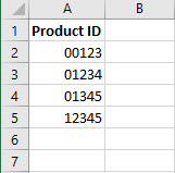
Another option is to format a cell with a 'Custom' format setting a specific number of characters, in order for this to be an options for the data length must be consistent. For example, if all of your ID's are 5 characters long and you input 1234 Excel will convert the number to a 5-character string making it 01234.
- Select the entire column where the leading zeros have been removed.
- Right click in the column and select cell format.
- Click the Number Tab and select Custom in the category section.
- In the Type field type 0 (zero) five times
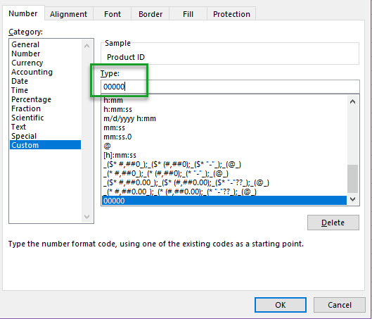
- Click OK
- Now type your number in to any field in the column, Excel will ensure that each number is at least 5 characters by padding with a 0 at the beginning of the number.